Using Basic Features of GLISTER

Getting Started with GLISTER Tutorials

Perhaps the best way to learn the basic features of GLISTER is to follow the tutorials included in the XMODEL installation package. The tutorial materials are located under the directory named $XMODEL_HOME/tutorial where $XMODEL_HOME denotes the XMODEL installation path. Each tutorial directory contains a README file and a /doc sub-directory containing the tutorial documentations in PDF format.

Currently, the following two tutorials cover GLISTER:

• $XMODEL_HOME/tutorial/glister_basic: a hands-on tutorial on how to compose analog models using GLISTER and run XMODEL simulations.
• $XMODEL_HOME/tutorial/xmodel_hslink: an in-depth tutorial on how to model various components of high-speed I/O interfaces and simulate their system-level performances with XMODEL and GLISTER.

For instance, to start with the glister_basic tutorial, first copy the tutorial package into your local directory (e.g. ~/glister_basic):

$ cp -R ${XMODEL_HOME}/tutorial/glister_basic ~/
$ cd ~/glister_basic

The tutorials assume that you have already set up XMODEL and GLISTER properly for your environment. If not, please refer to Chapter 1 of this document or the XMODEL Installation and Setup Guide for full details.

To define some additional environment variables used by the tutorial, source the proper setup script included in the tutorial depending on your shell type:

# for bash-like shells
$ source ~/glister/etc/setup.bashrc

# for csh-like shells
$ source ~/glister_basic/etc/setup.cshrc

Starting Cadence® Virtuoso®

GLISTER fully supports Cadence® IC 6.1.5 and later versions as well as Cadence® ICADV 12.1 and later versions. With Cadence® IC 5.1 products, however, not all the GLISTER features and functionalities may be available. This document will explain the features of GLISTER assuming the Cadence® IC 6.1.5 environment.

To start Cadence® Virtuoso®, type the following commands on your Linux command-line:

$ cd ~/glister_basic/cadence
$ virtuoso &

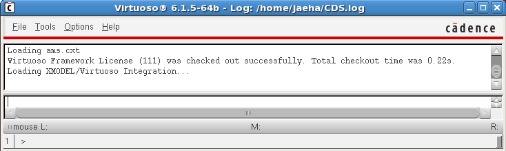
Figure 7. Cadence® Virtuoso® Command Interpreter Window (CIW)

Then, the Cadence® Virtuoso® Command Interpreter Window (CIW) will show up. This documentation will call it "CIW" in short. As a first step, try browsing the XMODEL primitives provided as symbols in the library named "xmodel_prims". To do so, select the Tools->Library Manager pull-down menu from the CIW. Once the Library Manager window is open, select the library named "xmodel_prims" and browse the cells contained in that library. There should be more than hundred cells, each of which corresponds to an XMODEL primitive.

One way to browse these XMODEL primitive cells easily is to check the Show Categories option box in the Library Manager as shown in Figure 8. Then, you can browse the XMODEL primitive cells by their categories, such as functions, circuits, stimuli, logic gates, variable domain translators (VDTs), connectors, and measurement probes. For further information on the XMODEL primitives and their categories, please refer to the XMODEL Reference Manual.

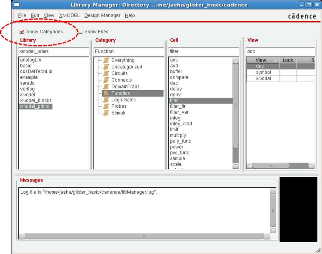
Figure 8. Browsing the available XMODEL primitives using Cadence® Virtuoso® Library Manager

Each cell in the "xmodel_prims" library has a "doc" view, which contains the on-line documentation on the corresponding XMODEL primitive. When you double-click on the "doc" view item from the Library Manager window, a web browser window will pop up and display the documentation. You can choose to use your favorite web browser by defining the Web Browser option available from the Options->User Preferences menu of the CIW. Please refer to the Cadence documentations if you’d like to load your browser choice upon start-up (e.g. setting the $CDS_DEFAULT_BROWSER environment variable).

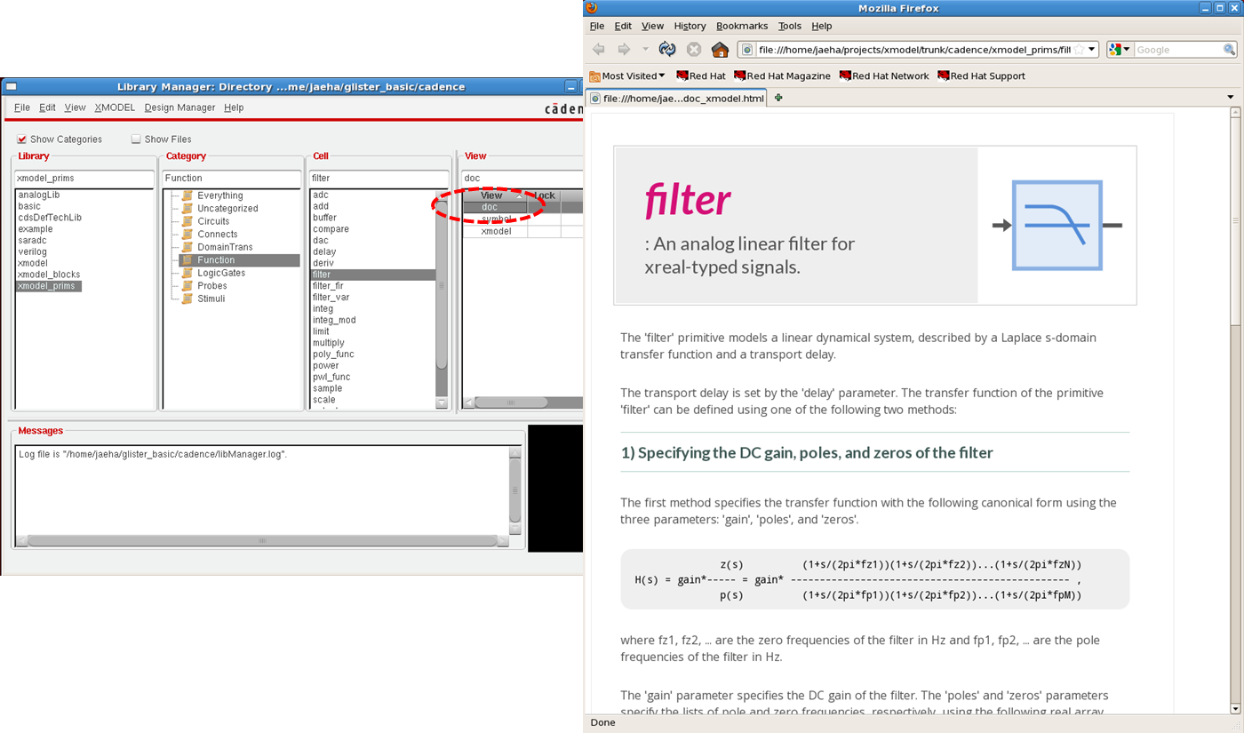
Figure 9. The on-Line documentations on XMODEL primitives accessible from the Cadence® Library Manager window via “doc” views.

Each cellview in the Cadence® design database is denoted by three fields: library name, cell name, and view name. This document will use the notation of <library>:<cell>:<view> to specify a cellview. For instance, a cellview named mylib:mycell:schematic corresponds to the schematic view of the cell named mycell included in the library mylib.

Composing Model Schematics

With GLISTER, you can compose XMODEL models for your circuits or systems in schematic forms. The procedure is basically equivalent to the procedure of composing schematics in the Cadence® Virtuoso® Schematic Editor using the XMODEL primitive symbols available from the "xmodel_prims" library as leaf cells. While this section will walk you through the basic steps of composing a model schematic using the Cadence® Virtuoso® Schematic Editor, you should refer to the Cadence® documentations for the full descriptions on its usages and features.

Opening an Existing Schematic Cellview

To open a schematic cellview existing in the design database, open the Library Manager window and select the library and cell names of the cellview to open and finally double-click on the view name (Figure 10). Then a new Cadence® Virtuoso® Schematic Editor window will pop-up and display the stored content of the cellview (Figure 11).

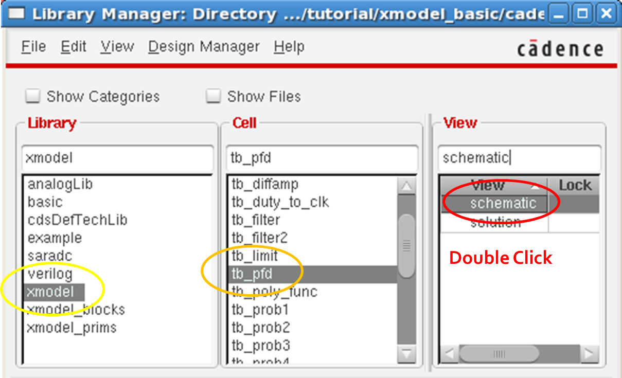
Figure 10. Opening an existing cellview.

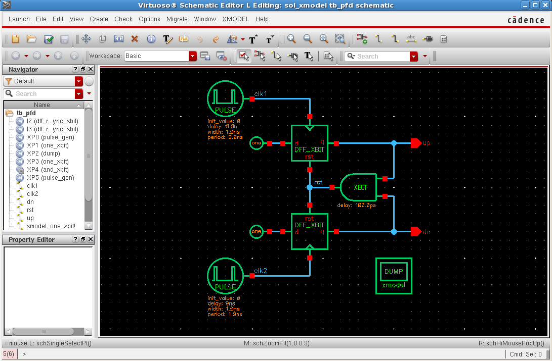
Figure 11. Cadence® Virtuoso® Schematic Editor window.

Creating a New Schematic Cellview

To create a new cellview from scratch, you can select either the File->New->Cellview menu from the CIW (Figure 12) or from the Library Manager window (Figure 13). Try creating a new schematic cellview named xmodel:tb_stim:schematic as illustrated in Figure 12 and Figure 13.

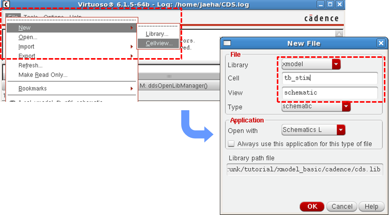
Figure 12. Creating a new cellview from the CIW.

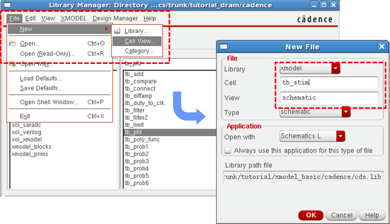
Figure 13. Creating a new cellview from the Library Manager.

Adding Instances and Wires

A minimal way of composing a model schematic is to add instances of the XMODEL primitives and connect them up using wires. This section will use a very simple example to illustrate the basic usage of the Cadence Virtuoso Schematic Editor.

An illustrative example shown in Figure 14 generates a sinusoidal signal using a sin_gen primitive and records it to a waveform file using a probe_xreal primitive. Thus, the example uses two instances and one wire connecting between the two.

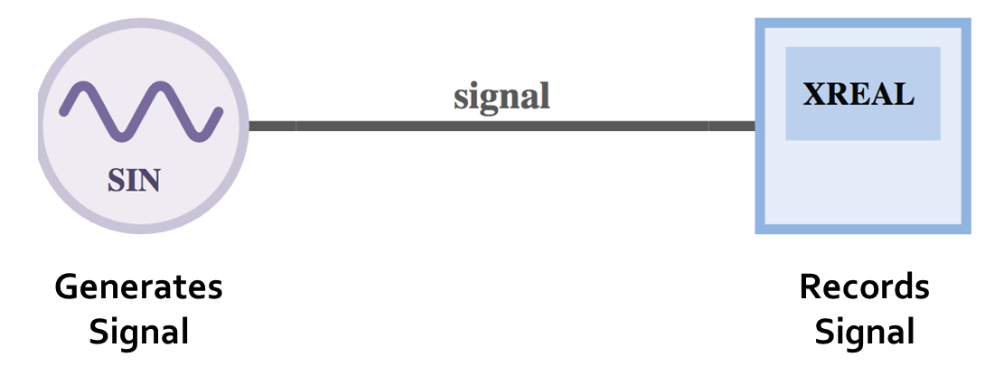
Figure 14. An illustrative example of composing a model schematic.

First, to add new instances on the schematic, use the following steps:

1. elect the Create->Instance pull-down menu or alternatively press "I" key on the schematic editor window. Then, the Add Instance window will pop up.
2. Select library, cell, and view of the instance you want to add (e.g. xmodel_prims:sin_gen:symbol).
3. Optionally, adjust the values of the parameters as desired.
4. On the schematic editor window, click the right mouse button where you want to place the instance.

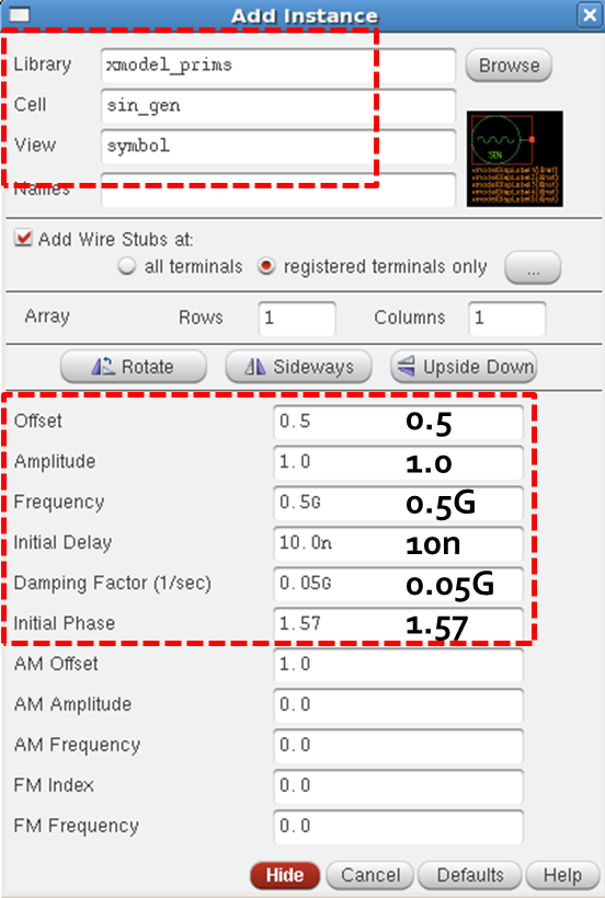
Figure 15. An example of adding an instance of sin_gen primitive to the schematic.

Second, to add wires connecting between the instances, use the following steps:

1. Select the Create->Wire menu or press "W" key on the schematic editor window.
2. Click the right mouse button once to mark the starting point of the wire and click twice to mark the ending point.
3. To add a label to the wire, select the Create->Wire Name menu or press "L" key.
4. When the Add Wire Name window pops up, enter the desired wire name and place the label on the wire by clicking the right mouse button on the wire.

Your final schematic may look like the one in Figure 16. Don’t forget to save your design by selecting the File->Check and Save menu, click the icon on the toolbar, or pressing "Shift + X" key.

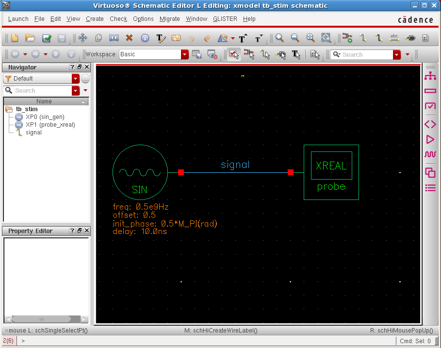
Figure 16. Finished schematic example.

Generating XMODEL Netlist

Once the schematic is checked and saved, you can generate its model netlist. To do so, select the GLISTER->Generate XMODEL Netlist pull-down menu available from the Cadence® Virtuoso® Schematic Editor window. Or, you can simply click the icon from the toolbar menu located on the right side of the schematic editor window. If you can’t find the GLISTER menu or toolbar on your schematic editor, please check if GLISTER is configured properly for your environment according to Section 2.1.

If the netlisting is finished successfully, you will see a success message displayed on the CIW. If you see any error or warning messages, you may have to fix the problems and try again. One of the common errors is not doing check-and-save after a change is made to the schematic.

To view the model netlists generated, you can select the GLISTER->Display XMODEL Netlist pull-down menu from the schematic editor window. Then, a text-editor window will pop-up showing the content of the model netlists as in Figure 17.

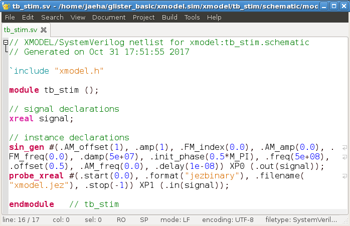
Figure 17. The generated model netlist for xmodel:tb_stim:schematic example.

It is noteworthy to check out the simulation directory which holds the generated model netlist files. By default, the location of the simulation directory is $XMODEL_SIMDIR/<library_name>/<cell_name>/<view_name>, where $XMODEL_SIMDIR is the environment variable defining the root location of the simulation directory as explained in Section 2.1, and <library_name>, <cell_name> and <view_name> denote the library, cell, and view names of the cellview netlisted, respectively. If the $XMODEL_SIMDIR environment variable is not defined, GLISTER uses $CDS_PROJECT/xmodel.sim as the default root location. If $CDS_PROJECT is not defined, then GLISTER uses $HOME/xmodel.sim. as the default root location of the simulation directory.

Once the netlisting is finished successfully, the simulation directory for the cellview contains the model files in SystemVerilog format as well as the other supporting files for running the simulation. For instance, the simulation directory for the xmodel:tb_stim: schematic example, of which full path information is provided in the CIW message when the netlisting is finished, may contain the following files:

• Makefile : a makefile script for running simulation
• tb_xmodel.mk : an alias to Makefile
• sources.f : a file containing a list of source files
• models/tb_stim.sv : a SystemVerilog source file containing the model netlist for xmodel:tb_stim:schematic cellview

Note that this directory contains all the necessary files to run the simulation. In fact, this directory structure is convenient for those who prefer running simulations on the command-line. For instance, one way to launch the XMODEL simulation is to execute the following commands on the Linux command line:

cd $XMODEL_SIMDIR/xmodel/tb_stim/schematic
make runsim

The Makefile script defines the target runsim with the option values such as the simulation time, simulation timescale, and others. For instance, an example Makefile for the xmodel:tb_stim:schematic cellview may look as below:

# Makefile ----------------------------------------------------------------
DEPEND_CELLVIEWS = xmodel:tb_stim:schematic
DEPEND_FILES =
SOURCES = -f sources.f
TOPMODULE = tb_stim

SIMTIME = 100ns
TIMESCALE = 1ps/1ps
SIMULATOR = ${XMODEL_SIMULATOR}
SIMOPTS =

all: runsim plotwave

runsim:
        xmodel $(SOURCES) --top $(TOPMODULE) --simtime $(SIMTIME) \
               --timescale $(TIMESCALE) --simulator $(SIMULATOR) $(SIMOPTS)

plotwave:
        xwave xmodel.jez --stdin

clean:
        xmodel --clean --simulator $(SIMULATOR)

These simulation options can be defined using the XMODEL Testbench Editor, which is explained next.

Running XMODEL Simulation

You can define the simulation options such as the SystemVerilog simulator, simulation time, simulation timescale, etc. using the XMODEL Testbench Editor. Select the GLISTER->Open Testbench Editor pull-down menu or click the icon from the toolbar. Then an XMODEL Testbench Editor window like the one in Figure 18 will pop up.

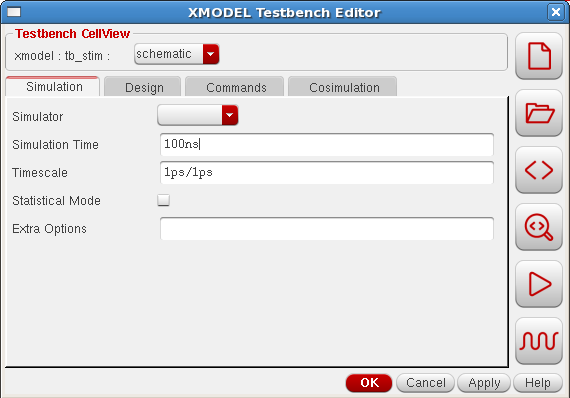
Figure 18. The XMODEL Testbench Editor window.

From this XMODEL Testbench Editor window, you can define various simulation options such as the SystemVerilog simulator of your choice (by default, it uses the one defined by the $XMODEL_SIMULATOR environment variable; please refer to the XMODEL Installation and Setup Guide for more information), simulation time, and simulation timescale in <time unit>/<time precision> notation used in Verilog. You can also define whether you want to perform statistical simulation or define extra options passed to the XMODEL Launcher (please refer to the XMODEL User Guide for more information).

You may find that the other tabs on the XMODEL Testbench Editor window (e.g. the Design, Commands, and Cosimulation tabs) are not enabled when you open the XMODEL Testbench Editor for a schematic cellview. Those tabs are available for defining an XMODEL testbench cellview, which is described in Section 4.4.

Once you set the simulation options, you can launch the XMODEL simulation simply by selecting the GLISTER->Run XMODEL Simulation pull-down menu or clicking the icon from the toolbar. Note that the XMODEL simulator and SystemVerilog simulator of your choice must be configured properly for your environment prior to performing this action. For further information, please refer to the XMODEL Installation and Setup Guide. As explained in Section 3.4, this action is equivalent to executing "make runsim" on the Linux command-line from the cellview’s simulation directory.

When you run the XMODEL simulations from the GLISTER environment, the output logs of the simulation will be displayed inside the Command Interpreter Window (CIW), as shown in Figure 19. The simulation is run in the background, so you can continue to use Cadence® Virtuoso® for other tasks. You may even run multiple XMODEL simulations from the same Cadence® Virtuoso® session.

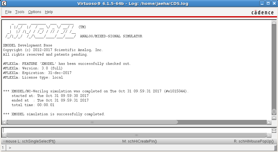
Figure 19. The Command Interpreter Window (CIW) displaying the output logs of the XMODEL simulation.

In case you need to stop the XMODEL simulations running in the background, you can select the GLISTER->Stop XMODEL Simulation pull-down menu. The action will kill all currently-running XMODEL simulations with the GLISTER environment.

Viewing Waveforms with XWAVE

Once the simulation is successfully completed, you can view the resulting waveforms using a waveform viewer. By default, GLISTER uses the XWAVE Waveform Viewer to plot the waveforms. You can use other waveform viewers of your choice by defining the proper options using the XMODEL Testbench Editor as explained in Section 4.4.

To view waveforms with the XWAVE Waveform Viewer, select the GLISTER->Open Waveform Viewer pull-down menu or click the icon on the toolbar menu. When the XWAVE Waveform Viewer window pops-up, you can select the signals of which waveforms you want to view by clicking the "+Add Signals" button on the bottom of the XWAVE window. Figure 20 shows a case of displaying the waveform from the xmodel:tb_stim:schematic example. Please refer to the XMODEL User Guide for more complete information on how to the XWAVE Waveform Viewer.

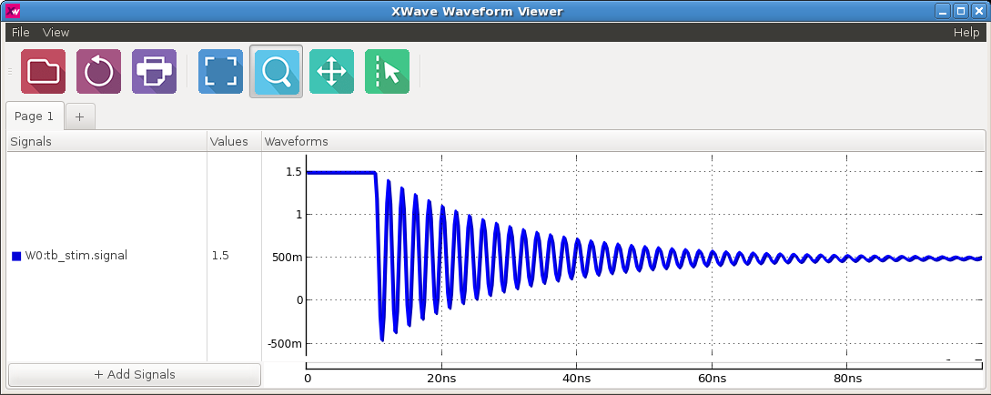
Figure 20. XWAVE Waveform Viewer displaying the simulated waveforms of the xmodel:tb_stim:schematic example.

GLISTER supports interactive probing with XWAVE. In other words, instead of selecting the signals to plot from the XWAVE’s Signal Browser, you can simply click on the signal located on the schematic to display its waveform. To enter into this interactive probing mode, select the GLISTER->Add Waveform Probe pull-down menu. You may notice that in this mode, your mouse cursor on the schematic editor screen changes, indicating that GLISTER is waiting for your selection. Simply click on the signals to view their waveforms. You can return to the normal schematic editing mode by pressing the ‘Esc’ key or by clicking on anywhere where no signal is located.

The wires of the signals that you select will be highlighted in different colors. In case you close the XWAVE Waveform Viewer and open it again by selecting the GLISTER->Open Waveform Viewer pull-down menu or clicking the icon while the signals remain highlighted, the selected waveforms will be automatically displayed on the new XWAVE Waveform Viewer window. If you want to de-select all the signals, select the GLISTER->Remove All Probes pull-down menu.