GLISTER-ADE Integration
Overview
Cadence® Virtuoso® Analog Design Environment (ADE) is the design and simulation environment widely used by Cadence® Virtuoso® users. This document explains how to use the features of GLISTER within the Cadence® Analog Design Environment (ADE).
Basically, this GLISTER-ADE integration allows you to choose “XMODEL” as a third-party simulator on the ADE session window, and perform various tasks including composing testbenches, generating netlists, running simulations, and viewing waveforms.
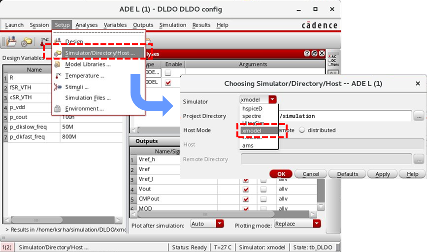
Figure 53. The GLISTER-ADE integration enables you to select “XMODEL” as a third- party simulator supported by Cadence® Virtuoso® ADE.
Please note that to use this GLISTER-ADE integration features, the users must have the proper OASIS licenses from Cadence® in addition to the Cadence® Virtuoso and ADE licenses and Scientific Analog’s GLISTER and XMODEL licenses. Please consult your Cadence® support when you get error messages regarding missing Cadence® licenses.
Configuring GLISTER-ADE Integration
Once you configure your Cadence® Virtuoso® environment for GLISTER as described in Section 2.1, you are ready to use the GLISTER-ADE integration features. However, if you have performed the configuration prior to the XMODEL 2018.03 Release and certain GLISTER-ADE features are not working for you, you may need to revisit the steps described in Section 2.1. Mainly, you will have to re-install the updated XMODEL registry files for the GLISTER-ADE integration as outlined below.
If you previously installed the XMODEL registry files into the Cadence® installation directory, execute the following command with the proper write privilege:
$XMODEL_HOME/bin/setup_registry --cdshome $CDSHOME
where $XMODEL_HOME environment variable defines the XMODEL installation path and the $CDSHOME environment variable defines the installation path of the Cadence® IC package. The old versions of Cadence® IC package (e.g. IC5.1) may use $CDS_INST_DIR instead of $CDSHOME.
If you previously installed the XMODEL registry files into your local directory, execute the following command to update the registry files:
cd $CDS_PROJECT or <your cadence work directory>
$XMODEL_HOME/bin/setup_registry --local .
The registry installer script setup_registry is introduced from the XMODEL 2018.03 Release. For certain registry files, such as data.reg, it may ask you to manually remove the prior XMODEL registry information contained within the file before proceeding. For more information, please refer to Section 2.1.
Using the ADE Setup Menu
The GLISTER-ADE integration supports the following action items in from the Setup pull-down menu of the ADE session window:
- Design
- Simulator/Directory/Host
- Model Libraries
- Temperature
- Stimuli
- Simulation Files
- Environment
Choosing the Simulator
To perform XMODEL simulation within ADE, first select the Setup->Simulator/Directory/Host menu item on the ADE session window and choose ‘xmodel‘ for the Simulator field as shown in Figure 54.

Figure 54. Choosing ‘xmodel‘ as the simulator in ADE.
On the same dialog window, you may define the location of the project directory. The project directory defines the root location of the XMODEL netlists and simulation results generated by the ADE sessions. The GLISTER-ADE integration follows the same convention with ADE in determining the simulation directory of a given cellview. For instance, the simulation directory for a cellview <libName>.<cellName>:<viewName> is located at <project directory>/<cellName>/xmodel/<viewName>. A simulation directory typically has two sub-directories: /netlist and /psf.
Selecting the Design
To select a design to be simulated, select the Setup->Design pull-down menu item as shown in Figure 55.
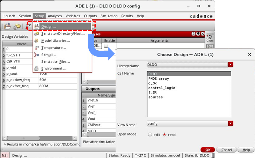
Figure 55. Selecting the design.
For XMODEL simulation, you can choose a cellview with two view types: schematic or config. For schematic-type cellviews, GLISTER performs the netlisting based on the Switch View List and Stop View List environment options defined for this ADE session. For config-type cellviews, GLISTER performs the netlisting as specified by its hierarchy configuration information.
Defining the Environment Options
To define various environment options for the ADE session, select the Setup->Environment pull-down menu item as shown in Figure 56.
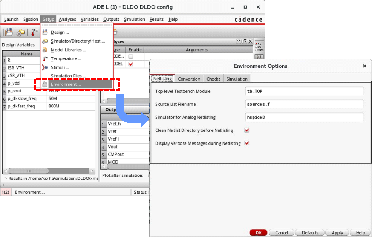
Figure 56. Defining the environment options.
The Environment Options dialog window has four tabs: Netlisting, Conversion, Checks, and Simulation. These options control the netlisting and simulation performed by GLISTER and XMODEL. The following tables describe the available options on each tab.
Table 5. GLISTER-ADE environment options on the Netlisting tab.
| Option Name | Description |
| Switch View List | List of views that GLISTER can select for hierarchy traversal during netlisting. This option is not used when the selected design is a config-type cellview. |
| Stop View List | List of views at which the GLISTER netlister stops traversing the hierarchy. This option is not used when the selected design is a config-type cellview. |
| Top-level Testbench Module | Name of the top-level testbench module defining the design variables, stimuli, DUT instance, and waveform recording (default: tb_TOP). |
| Source List File Name | Name of the file containing the list of model files generated by the GLISTER netlister (default: sources.f). |
| Simulator for Analog Netlisting | The format of the analog simulation (SPICE) netlist. When the GLISTER netlister meets a part of design that can only be netlisted using an analog netlister, it creates netlists suitable for mixed-mode simulation. Valid values include: hspiceD, spectre, and veriloga. |
| Clean Netlist Directory before Netlisting | If this option is checked, the netlist directory will be cleaned before netlisting. |
| Display Verbose Messages during Netlisting | If this option is checked, verbose messages will be displayed on CIW during netlisting. |
Table 6. GLISTER-ADE environment options on the Type Conversion tab.
| Option Name | Description |
| Default Conversion Level for Logic 1 | Default conversion level for logic 1 when a digital type signal (e.g., xbit or bit) is converted to an analog type signal (e.g., xreal or real). This value takes precedence over the value of the xmodelConvLevel1 SKILL variable. |
| Default Conversion Level for Logic 0 | Default conversion level for logic 0 when a digital type signal (e.g., xbit or bit) is converted to an analog type signal (e.g., xreal or real). This value takes precedence over the value of the xmodelConvLevel1 SKILL variable. |
| Default Conversion Thresholds for Logic 1 | Default conversion threshold for logic 1 when an analog type signal (e.g., xreal or real) is converted to a digital type signal (e.g., xbit or bit). This value takes precedence over the value of the xmodelConvThres1 SKILL variable. |
| Default Conversion Thresholds for Logic 0 | Default conversion threshold for logic 0 when an analog type signal (e.g., xreal or real) is converted to a digital type signal (e.g., xbit or bit). This value takes precedence over the value of the xmodelConvThres0 SKILL variable. |
| Default Driving Strength (0~7) | Default driving strength assumed when an analog type signal (e.g., xreal or real) is converted to a digital type signal (e.g., xbit or bit). The possible choices are the integer values from 0 to 7 (4: weak, 5: pull, 6: strong, 7: supply). This value takes precedence over the value of the xmodelConvStrength SKILL variable. |
Note that the bit type denoted in the context of this documentation refers to the four-value logic type in Verilog, which is equivalent to the wire, reg, or logic types.
Table 7. GLISTER-ADE environment options on the Checks tab.
| Option Name | Description |
| Check Port Directions | If it is checked, GLISTER will check any conflicts between the directions of the ports connected during netlisting. |
| Check Signal Types | If it is checked, GLISTER will check any conflicts between the signal types of the ports connected during netlisting. |
| Check Bus Names | If it is checked, GLISTER will check any conflicts between the names of the signals sharing the same bus during netlisting. |
Table 8. GLISTER-ADE environment options on the Simulation tab.
| Option Name | Description |
| User Command-Line Options | User-defined options to be added to the simulation run command (make runsim). |
| Automatic Output Log | If it is checked, the simulation output log will be displayed while a simulation is running. |
| Macro Definitions | Define macros passed to the Verilog simulator. This option is equivalent to the --define option of the xmodel launcher command. |
| Elaborator Options | Define vendor-specific options passed to the Verilog elaborator. This option is equivalent to the --elab- option <OPTIONS> -- option of the xmodel launcher command. |
| Simulator Options | Define vendor-specific options passed to the Verilog simulator. This option is equivalent to the --sim- option <OPTIONS> -- option of the xmodel launcher command. |
| Binary Architecture | Binary architecture of the SystemVerilog simulator Binary Architecture performing the XMODEL simulation. Possible modes are Auto (default), 64bit, and 32bit. |
Defining Testbench Stimuli
Cadence® ADE lets you define stimuli waveforms applied to the design to be simulated, providing a convenient way of composing simple types of testbenches. The GLISTER-ADE integration supports the same capability for XMODEL simulations. You can define stimuli waveforms in either of the following two ways:
- Setting up stimuli from the Setup->Stimuli menu
- Specifying a SystemVerilog file defining the stimuli from the Setup->Simulation Files menu.
Defining Stimuli Using the Setup->Stimuli Menu
One way to define stimuli waveforms is to select the Setup->Stimuli pull-down menu item or click the ![]() icon located on the top toolbar of the ADE session window (Figure 57).
icon located on the top toolbar of the ADE session window (Figure 57).
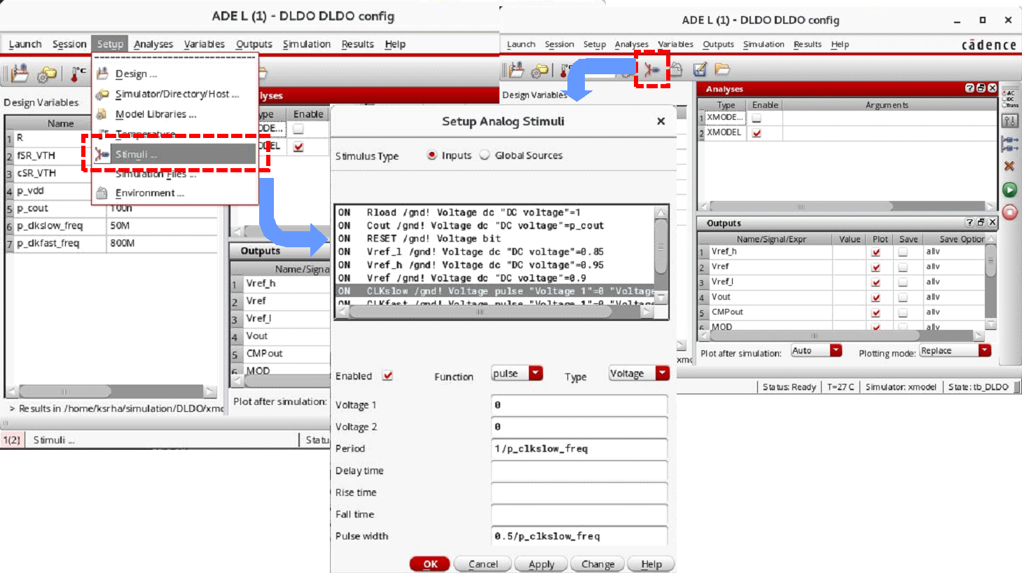
Figure 57. Defining stimuli using the Setup->Stimuli menu.
When the Setup Analog Stimuli dialog window appears, you can assign a stimulus source to each input port of the design by choosing one of the following functions listed in Table 9. The Type field in the Setup Analog Stimuli dialog window defines whether the stimulus drives the voltage or current of the input port.
Table 9. List of stimulus functions available from the Setup Analog Stimuli dialog window.
| Function Name | Description |
| dc | Add a dc_gen XMODEL primitive as a stimulus source, which generates an xreal-type, constant analog signal. |
| sin | Add a sin_gen XMODEL primitive as a stimulus source, which generates an xreal-type, sinusoidal signal. |
| exp | Add a exp_gen XMODEL primitive as a stimulus source, which generates an xreal-type, exponential signal. |
| pwl | Add a pwl_gen XMODEL primitive as a stimulus source, which generates an xreal-type, piecewise-linear (PWL) signal. |
| pulse | Add a pulse_gen XMODEL primitive as a stimulus source, which generates an xbit-type, digital pulse with specified pulse width and period. |
| bit | Add a pat_gen XMODEL primitive as a stimulus source, which generates an xbit-type bit sequence with a fixed pattern. |
| prbs | Add a prbs_gen XMODEL primitive as a stimulus source, which generates an xbit-type, digital pseudo-random bit sequence (PRBS). |
Digital-Type Stimulus Functions
The stimulus functions pulse, bit, and prbs define stimulus waveforms of digital types and the GLISTER-ADE integration uses the pulse_gen, pat_gen, and prbs_gen primitives of XMODEL to describe their waveforms, respectively. Please refer to the XMODEL Reference Manual for more detailed descriptions on these XMODEL primitives.
The following Table 10, Table 11, and Table 12 list the parameters available from the Setup Analog Stimuli dialog window for the pulse, bit, and prbs stimulus functions, respectively.
Note that these digital-type stimulus functions can also drive analog-type input ports, such as xreal and real type ports. In such cases, the digital values of the stimulus waveform will be converted to analog values according to the parameter values defining the corresponding conversion levels (e.g. One value, Zero value, Rise time, and Fall time).
When a digital-type stimulus function drives a digital-type input port (e.g. xbit or bit type port), it can only be a voltage type. However, when the stimulus function drives an analog-type input port (e.g. xreal or real type port), it can either be a voltage type or current type.
Table 10. Available parameters for the pulse stimulus function.
| Parameters | Description |
| Voltage 1 | Voltage level #1 that sets the initial level of the pulse (must be 0 or 1 for digital-type signals). |
| Voltage 2 | Voltage level #2 (must be 0 or 1 for digital-type signals). |
| Delay time | Initial delay of the pulse. |
| Pulse width | Width of the pulse at the voltage level #2. |
| Period | Repetition period of the pulse. |
| Rise time | Transition time from voltage level #1 to #2 (used only for analog-type signals). |
| Fall time | Transition time from voltage level #2 to #1 (used only for analog-type signals). |
Table 11. Available parameters for the bit stimulus function.
| Parameters | Description |
| Pattern Parameter data | Bit pattern data defined using a string of binary digits (e.g. 10110100). |
| Pattern Parameter rptstart | The position in the bit pattern data where the repetition starts. |
| Pattern Parameter rpttimes | The number of repetitions to be generated. |
| Delay time | Initial delay of the bit sequence. |
| Period | Time period of each bit. |
| One value | Conversion level of logic 1 (used only for analog-type signals). |
| Zero value | Conversion level of logic 0 (used only for analog-type signals). |
| Rise time | Transition time from logic 0 to logic 1 (used only for analog-type signals). |
| Fall time | Transition time from logic 1 to logic 0 (used only for analog-type signals). |
Table 12. Available parameters for the prbs stimulus function.
| Parameters | Description |
| LFSR Mode | The length (N) of the linear-feedback shift register (LFSR) generating a pseudo-random bit sequence (PRBS) of 2^N-1. Supported values are PN3~PN128. |
| Delay time | Initial delay of the bit sequence. |
| Bit period | Time period of each bit. |
| One value | Conversion level of logic 1 (used only for analog-type signals). |
| Zero value | Conversion level of logic 0 (used only for analog-type signals). |
| Rise time | Transition time from logic 0 to logic 1 (used only for analog-type signals). |
| Fall time | Transition time from logic 1 to logic 0 (used only for analog-type signals). |
Note that the pat_gen and prbs_gen primitives describing the stimulus functions bit and prbs require a trigger input, indicating the time period and initial delay of the data pattern being generated. To generate such trigger inputs, the GLISTER-ADE integration uses the pulse_gen primitives..
Analog-Type Stimulus Functions
The rest of stimulus functions listed in Table 9, including dc, sin, exp, and pwl, define stimulus waveforms of analog types. The Type field defines whether the stimulus function drives the voltage or current of the input port. Note that these analog-type stimulus functions cannot drive a digital-type input port (e.g. xbit or bit type port).
The following tables (Table 13, Table 14, Table 15, and Table 16) list the parameters available for the dc, sin, exp, and pwl stimulus functions, most of which directly correspond to the parameters of the dc_gen, sin_gen, exp_gen, and pwl_gen primitives, respectively. Please refer to the XMODEL Reference Manual for more detailed descriptions on these primitives.
Table 13. Available parameters for the dc stimulus function.
| Parameters | Description |
| DC voltage/current | DC value. |
Table 14. Available parameters for the sin stimulus function.
| Parameters | Description |
| Delay time | Initial delay. |
| Offset voltage/current | Offset value. |
| Amplitude | Amplitude of the base sinusoid. |
| Initial phase for Sinusoid | Initial phase of the base sinusoid. |
| Frequency | Frequency of the base sinusoid. |
| Damping factor | Damping factor for exponentially-decaying amplitude. |
| AM modulation index | Modulation index of single-frequency amplitude modulation. |
| AM modulation frequency | Modulation frequency of single-frequency amplitude modulation. |
| FM modulation index | Modulation index of single-frequency frequency modulation. |
| FM modulation frequency | Modulation frequency of single-frequency frequency modulation. |
Table 15. Available parameters for the exp stimulus function.
| Parameters | Description |
| Voltage/Current 1 | Initial value of the first exponential waveform. |
| Voltage/Current 2 | Final value that the first exponential waveform converges to at time of infinity. |
| Delay time 1 | Delay of the first exponential waveform. |
| Delay time 2 | Delay of the second exponential waveform. |
| Damping factor 1 | Time constant of the first exponential waveform. |
| Damping factor 2 | Time constant of the second exponential waveform. |
Table 16. Available parameters for the pwl stimulus function.
| Parameters | Description |
| Delay time | Initial delay of the PWL waveform. |
| Period of the PWL | Period at which the PWL waveform is repeated. |
| Number of pairs of points | Number of time-value pairs defining the PWL waveform. |
| Time 1, 2, 3, … | Series of time points defining the PWL waveform. |
| Voltage/Current 1, 2, 3, … | Series of value points defining the PWL waveform. |
Automatic Type Coercion for Stimuli
The stimulus sources described in the previous subsection produce either xreal or xbit type outputs. In case the input ports to which you are assigning the stimulus functions do not have the matching signal types, the GLISTER-ADE integration automatically inserts the proper connect primitives and performs type coercion. When these type-coercing connect primitives have to convert digital signals into analog ones, the GLISTER-ADE integration uses the conversion levels defined for the stimulus function. Please refer to Section 4.2 for the automatic type detection and coercion capability of GLISTER and XMODEL Reference Manual for the available connect primitives.
Defining Stimuli with a Stimulus File
The other way of defining the testbench stimuli is to specify a stimulus file that lists the stimulus description in SystemVerilog format directly. The contents of this stimulus file will be inserted into the final testbench file composed by the GLISTER-ADE integration.
To add a stimulus file, select the Setup->Simulation Files pull-down menu from the ADE session window. When the Simulation Files Setup dialog window shows up, you can add definitions for the Include Paths, Definition Files, and Stimulus Files. The entries in the Include Paths and Definition Files will be added to the source list file (by default, sources.f). The contents of the files listed in the Stimulus Files will be inserted into the testbench file composed by the GLISTER-ADE integration.
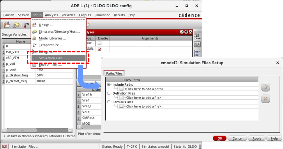
Figure 58. Defining stimuli by specifying stimulus files.
Note that defining testbench stimuli using both the Setup->Stimuli menu and Setup->Simulation Files menu may result in duplicate definitions for the same signals and cause an error during the simulation.
Using the ADE Analysis Menu
The GLISTER-ADE integration supports the following action items in from the Analysis pull-down menu of the ADE session window:
- Choose
- Delete
- Enable
- Disable
Choosing the Simulation Analysis
The GLISTER-ADE integration supports two types of simulation analysis: ‘XMODEL‘ and ‘XMODEL+SPICE‘. The ‘XMODEL‘ analysis corresponds to an XMODEL simulation using a SystemVerilog simulator only. The ‘XMODEL+SPICE‘ analysis corresponds to a co- simulation between XMODEL and SPICE using a mixture of SystemVerilog models and SPICE/Spectre netlists.
Unlike SPICE which supports a variety of analysis modes such as DC and AC analyses in addition to the transient (TRAN) analysis, all simulation analyses performed by XMODEL supports only transient, time-domain simulations. Also, you can choose only one analysis for each ADE session.
To choose a simulation analysis, select the Analyses->Choose pull- down menu item from the ADE session window (or click the ![]() icon on the right-hand-side toolbar). From the Analysis Editor dialog window that pops up, you can choose either ‘XMODEL‘ or ‘XMODEL+SPICE‘ as the simulation analysis (Figure 59).
icon on the right-hand-side toolbar). From the Analysis Editor dialog window that pops up, you can choose either ‘XMODEL‘ or ‘XMODEL+SPICE‘ as the simulation analysis (Figure 59).
The choice of the analysis between ‘XMODEL‘ and ‘XMODEL+SPICE‘ affects the behavior of the GLISTER netlister. When ‘XMODEL‘ is chosen, it is assumed that the design consists only of SystemVerilog models and the GLISTER netlister flags an error when it encounters a part of the design that can only be netlisted in an analog simulator format (SPICE or Spectre). On the other hand, when ‘XMODEL+SPICE‘ is selected, the GLISTER netlister prepares a mixture of SystemVerilog models and SPICE/Spectre netlists suitable for an XMODEL-SPICE cosimulation for the same case.
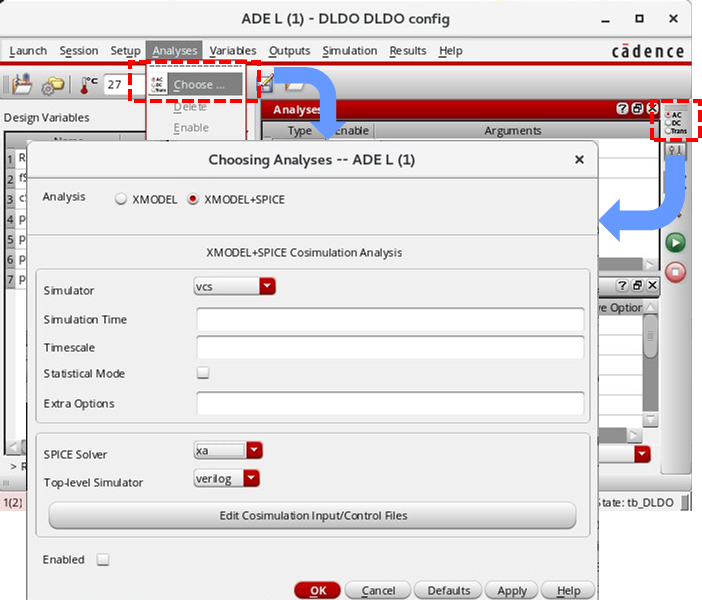
Figure 59. Choosing the simulation analysis.
Table 17 and Table 18 below describe the options available for the ‘XMODEL‘ and ‘XMODEL+SPICE‘ analyses on the Analysis Editor dialog window.
Table 17. GLISTER-ADE analysis options available both for the ‘XMODEL‘ and ‘XMODEL+SPICE‘ analyses.
| Option Name | Description |
| Simulator | SystemVerilog simulator to be used. Possible values are: ncverilog, vcs, and modelsim. |
| Simulation Time | Specify the duration of the simulation to run. |
| Timescale | Specify the simulation timescale and precision in Verilog format, such as 1ps/1ps. |
| Statistical Mode | Enable statistical simulation. When it is enabled, XMODEL computes the statistical properties of time-varying noises and jitters during simulation. |
| Extra Options | Additional options passed to the xmodel launcher command. |
Table 18. GLISTER-ADE analysis options available only for the ‘XMODEL+SPICE‘ analysis.
| Option Name | Description |
| SPICE Solver | SPICE simulator to be used for simulating the design parts netlisted in the analog (SPICE/Spectre) format. Note that the SPICE Netlist Format option in Table 5 specifies the netlist format, while this option specifies the simulator). For vcs as the SystemVerilog simulator, finesim, hsim, and xa are supported. For ncverilog, |
| Top-level Simulator | Specify whether the top-level simulator is verilog or spice. Currently, GLISTER supports only Verilog-top configuration. |
| Edit Cosimulation Input/Control Files | Open a dialog form to edit the SPICE simulator input file and cosimulation control file. |
For the 'XMODEL+SPICE' analysis, you can click on the Edit Cosimulation Input/Control Files button to open the Edit Cosimulation Input/Control Files dialog window (Figure 60). This dialog window has two tabs: the SPICE Simulator Input File tab and Cosimulation Control File tab. From the SPICE Simulator Input File tab, you can define the content of the input file fed to the SPICE simulator and from the Cosimulation Control File tab, you can define the content of the co-simulation control file. For more description regarding these files and the macros used for describing their contents (e.g. $(SIMTIME)), please refer to Section 4.6.
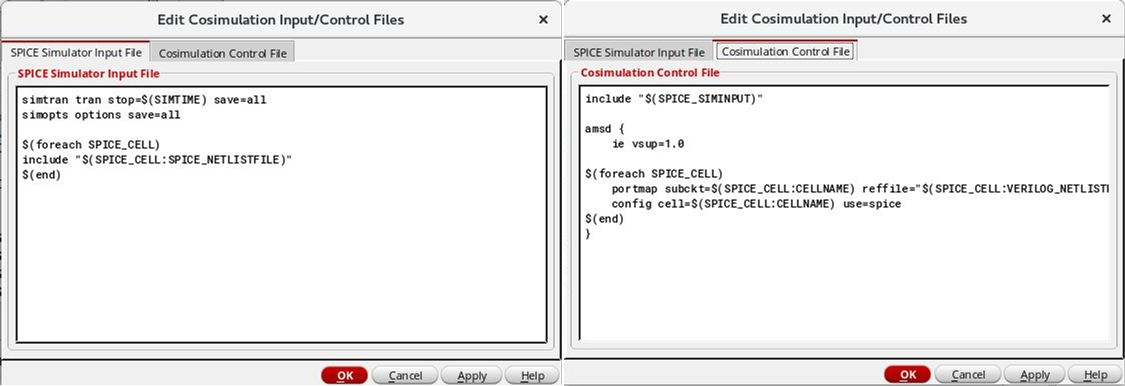
Figure 60. The SPICE Simulator Input File tab and Cosimulaton Control File tab of the Edit Cosimulation Input/Control Files dialog window.
Specifying Model Libraries and Temperature for SPICE/Spectre Simulation
When the 'XMODEL+SPICE' analysis is chosen, the model file definitions you can add from the Setup->Model Libraries menu and the temperature you can define from the Setup->Temperature menu will be prepended to the final input file for the SPICE simulator.
On the other hand, the two options have no effects when the 'XMODEL' analysis is selected.
Using the ADE Variables Menu
The GLISTER-ADE integration supports the following action items in from the Variables pull-down menu of the ADE session window:
- Edit
- Delete
- Find
- Copy From Cellview
- Copy To Cellview
Defining Design Variables
Often, it is more convenient to set the parameter values of the design to be simulated or the testbench stimuli using a set of design variables rather than using direct numerical values. For instance, the parameters of multiple stimulus sources may be related to some common numbers such as the operating frequency or supply voltage. In this case, using design variables offers a reliable way to keep the parameter values consistent especially when one needs to update them frequently.
In the context of XMODEL simulation, the design variables defined within the ADE session correspond to the global parameters (i.e. parameters not belonging to any SystemVerilog modules). Hence, the design variables can be used for defining the parameters of the testbench stimuli as well as those of the design to be simulated. Note that the parameters in SystemVerilog must have constant values which can be resolved during the elaboration stage of the simulation.
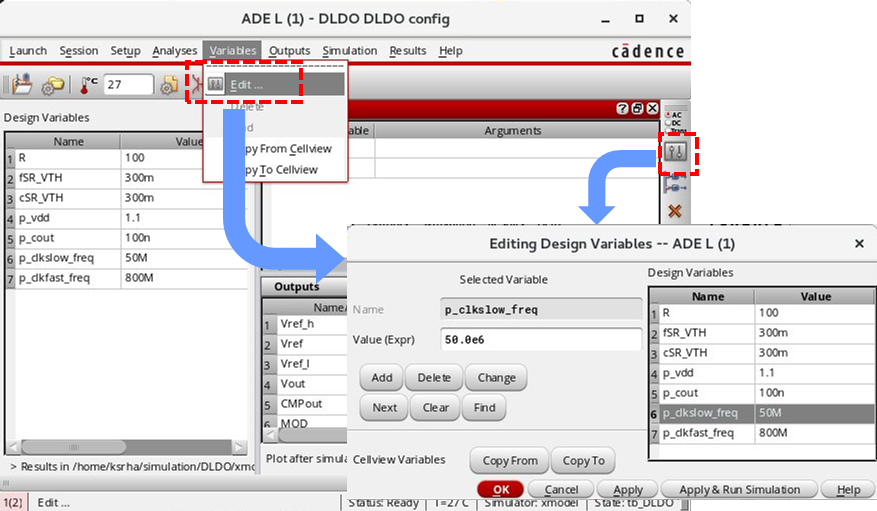
Figure 61. Defining design variables.
You can define design variables by selecting the Variables->Edit pull- down menu item or by clicking the ![]() icon located on the right toolbar of the ADE session window (Figure 61).
icon located on the right toolbar of the ADE session window (Figure 61).
Figure 62 shows an illustrative example of using the design variables. A design variable named p_clkslow_freq is defined with a value of 50M, which is referenced in the parameter field expressions for a pulse stimulus function assigned to the input port named CLKslow.
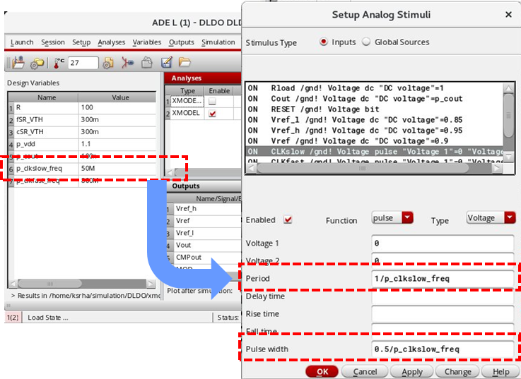
Figure 62. An illustrative example of using design variables.
Using the ADE Outputs Menu
The GLISTER-ADE integration supports the following action items in from the Outputs pull-down menu of the ADE session window:
- Setup
- Delete
- Import
- Export
- To Be Saved
- To Be Plotted
- Output Options
Setting Outputs
You can specify the signals of which simulated waveforms are to be saved or to be plotted. The GLISTER-ADE integration will then record the waveforms of the signals to be saved and plot the waveforms of the signals to be plotted using a waveform viewer (e.g. XWAVE) after the simulation is run.
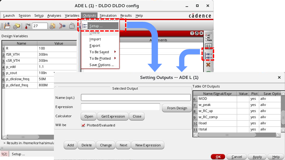
Figure 63. Setting outputs.
To specify the signals to be saved or plotted, select the Outputs->Setup pull-down menu or click the ![]() icon located on the right toolbar of the ADE session window. When the Setting Outputs dialog window appears, you can select a signal to be saved or to be plotted either by entering its name or by selecting it from the schematic after clicking the From Design button (Figure 63).
icon located on the right toolbar of the ADE session window. When the Setting Outputs dialog window appears, you can select a signal to be saved or to be plotted either by entering its name or by selecting it from the schematic after clicking the From Design button (Figure 63).
Each signal selected to be saved or plotted is listed in the Outputs pane of the ADE session window, where you can modify the selections of its Plot or Save check boxes (Figure 64). The signal selections can also be imported from or exported to a CSV (comma- separated values) file using the Outputs->Import and Outputs->Export pull-down menus of the ADE session window.
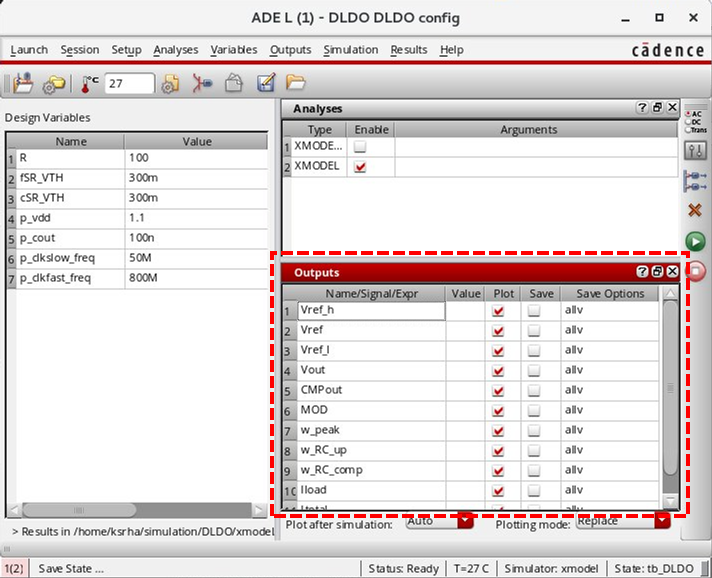
Figure 64. The Outputs pane of the ADE session window.
Note that the current version of GLISTER-ADE integration does not support saving or plotting currents flowing into the ports. Also, it does not yet support saving or plotting derived signals using expressions.
Setting Saving Options
You can control the way the GLISTER-ADE integration saves or plots the signal waveforms by selecting the Outputs->Saving Options pull- down menu on the ADE session window (Figure 65). Table 19 describes the available options listed in the Saving Options dialog window.
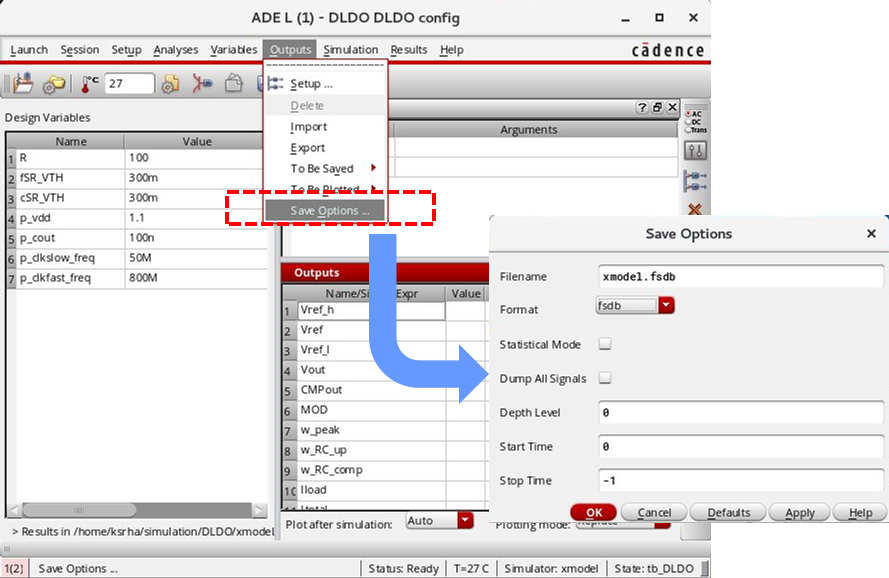
Figure 65. Setting saving options.
Table 19. List of available options in the Output Options dialog window.
| Parameters | Description |
| Filename | Name of the waveform file. |
| Format | Format of the waveform file. Supported format is jezbinary, jezascii, and fsdb. The JEZ format is the Scientific Analog's proprietary format that best preserves the event-driven signal waveforms of XMODEL. The jezbinary format stores the data in binary format and jezascii stores in ASCII format. The fsdb format is compatible with the one produced by Synopsys® Verdi (FSDB). |
| Statistical Mode | A flag to enable/disable statistical data recording. It is available only for JEZ format. |
| Dump All Signals | When selected, all the signals within the specified hierarchy depth level will be recorded to the waveform file. |
| Depth Level | Level of monitoring depth. For instance, a level of 1 means the top level only and level of 2 means the top level and one hierarchy level below. A level of 0 means all hierarchy levels. |
| Start Time | Absolute time to start the waveform recording. |
| Stop Time | Absolute time to stop the waveform recording. If its value is -1, the waveform will be recorded til the end of the simulation. |
Using the ADE Simulation Menu
The GLISTER-ADE integration supports the following action items in from the Simulation pull-down menu of the ADE session window:
- Netlist and Run
- Run
- Stop
- Netlist
Generating Netlists
You can create the model netlists and testbench files based on the specified stimuli, analyses, variables, and outputs by selecting the Simulation->Netlist->Create pull-down menu of the ADE session window. You can view the generated netlists by selecting the Simulation->Netlist->Display pull-down menu (Figure 66).
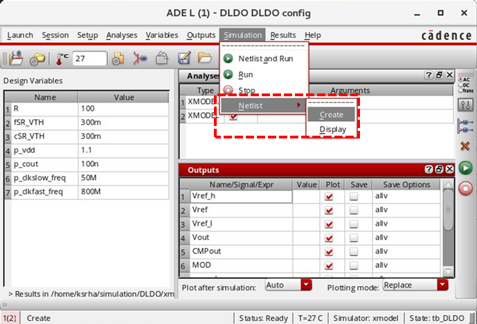
Figure 66. Generating netlists using the Simulation pull-down menu of the ADE session window.
The GLISTER-ADE integration mainly performs the following two actions when netlisting is launched. First, it calls the GLISTER netlister to generate the model netlists of the design itself. Depending on whether the selected analysis is 'XMODEL' or 'XMODEL+SPICE', the netlister produces SystemVerilog-only netlists or XMODEL-SPICE co-simulation netlists. The GLISTER netlister also creates the supporting files for simulation including the source list file (by default, sources.f) and Makefile script reflecting the options set using the Environment Options window (Table 8) and the Analysis Editor window (Table 17). For more information on the basic operation of this GLISTER netlister, please refer to Section 3.4.
Second, the GLISTER-ADE integration creates the top-level SystemVerilog testbench module based on the stimuli, variables, and outputs defined for the current ADE session.
The generated netlists, testbench, and other supporting files will be stored in a directory named <project directory>/<cellName>/xmodel/<viewName> where the <libName>, <cellName>, and <viewName> are the library, cell, and view names of the design cellview chosen by the Setup->Design pull- down menu, respectively. Please refer to Section 5.3 for more information about these pull-down menus.
Running Simulation
To run the simulation with the generated model netlists and testbench, select the Simulation->Run pull-down menu or click the ![]() icon located on the right toolbar of the ADE session window (Figure 67). When the Automatic Output Log environment option is enabled (see Table 8), you can check the progress of the simulation on a log monitor window.
icon located on the right toolbar of the ADE session window (Figure 67). When the Automatic Output Log environment option is enabled (see Table 8), you can check the progress of the simulation on a log monitor window.
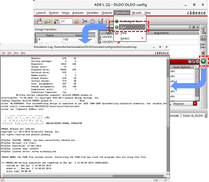
Figure 67. Running XMODEL simulation.
You can force the simulation to stop by selecting the Simulation->Stop pull-down menu or clicking the ![]() icon located on the right toolbar of the ADE session window.
icon located on the right toolbar of the ADE session window.
Using the ADE Results Menu
The GLISTER-ADE integration supports the following action items in from the Results pull-down menu of the ADE session window:
- VIVA
- XWAVE
- Log
Plotting Waveforms
Once the simulation is complete, you can check the results by plotting the simulated waveforms. The GLISTER-ADE integration currently supports the use of two waveform viewers within the ADE session window: XWAVE and VIVA, the Cadence® Virtuoso® Visualization and Analysis program. Note that the waveform files stored in JEZ format can be viewed only by XWAVE while the waveform files in FSDB format can be viewed by either XWAVE or VIVA.
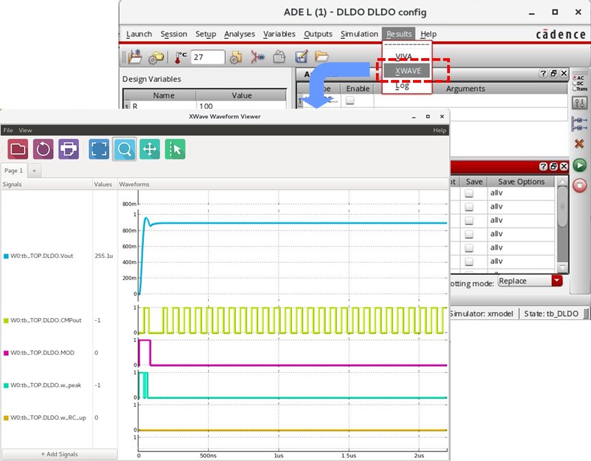
Figure 68. Viewing simulated waveforms using XWAVE.
To plot the simulated waveforms with XWAVE, select the Results->XWAVE pull-down menu (Figure 68). Please refer to the XMODEL User Guide for the information on the XWAVE waveform viewer.
On the other hand, to plot the simulated waveforms with Cadence® VIVA, select the Results->VIVA pull-down menu of the ADE session window (Figure 69). Please refer to the proper Cadence® documentations for the information on how to use VIVA.
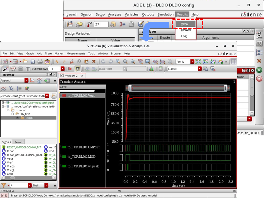
Figure 69. Viewing simulated waveforms using Cadence® VIVA.
Viewing Logs
XMODEL simulation also produces an output log, which may have been displayed to the log monitoring window during the simulation. You can view this output log again by selecting the Results->Log pull-down menu of the ADE session window.