Circuit Level Modeling with XMODEL
Overview
The Circuit-Level Modeling (CLM) feature of XMODEL allows one to describe electrical circuits as conservative system models carrying voltages and currents. In most behavioral simulators including XMODEL, the most basic way is to describe them as signal-flow system models.
In signal-flow systems, information propagates only in one direction from input to output. In such systems, the output of each signal-flow model is computed explicitly from its inputs. This is well suited for modeling systems consisting of blocks as shown in Figure 1. In fact, all digital behavioral models described in Verilog or VHDL are signal-flow models. Most modern HDL simulators exploit the unidirectional flow property of signal-flow models in performing the efficient event-driven simulation.
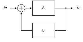
Figure 1. A signal-flow system model.
On the other hand, in conservative system models, there is no explicit definition of the directions in which signals propagate. For instance, an electrical circuit formed as a network of circuit elements is an example of conservative systems. A circuit has node voltages and branch currents that describe its states, of which influence may propagate in any directions in the network. The voltages and currents are determined according to laws of physics such as Kirchoff’s Voltage Law (KVL) and Current Law (KCL). The circuit simulation is typically performed by implicitly solving a set of equations governing these state variables of the system.
While XMODEL provides a rich set of primitives, we understand that it may not be always easy to describe all analog/mixed-signal circuits only as signal-flow models. One example is a switched-capacitor DC-DC converter shown in Figure 2, consisting of capacitors and switches that turn on and off periodically. Another example is an amplifier with a loading effect, of which output voltage is not only a function of the input voltage but also of the output load current. For these examples, it would be more straightforward to describe them as conservative systems, i.e. electrical circuits.
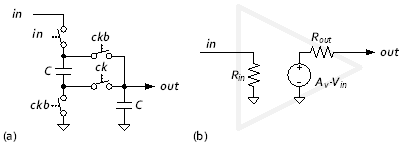
Figure 2. Examples of conservative system models of electrical circuits: (a) a switched-capacitor DC-DC converter and (b) a linear amplifier with loading effect (i.e. finite input and output resistances).
The XMODEL’s CLM feature allows one to describe circuits as conservative system models. For instance, Figure 3 lists the model for the switched-capacitor DC-DC converter in Figure 2, using the CLM feature in XMODEL. The model is essentially a structural netlist of the circuit itself. Yet, the simulation can be still run in the same event-driven fashion with the other XMODEL primitives, which is faster than the most SPICE simulators using the ordinary differential equation (ODE) solvers.
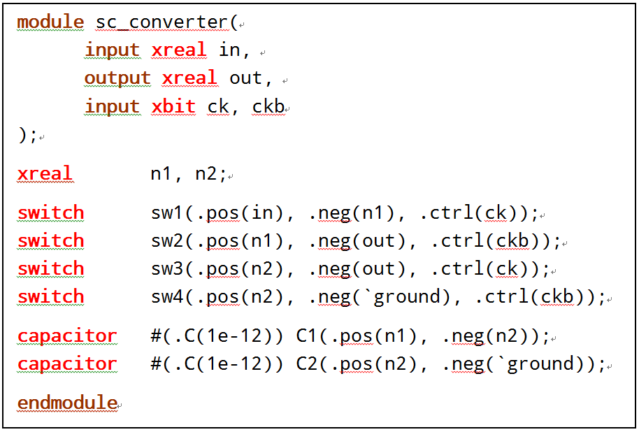
Figure 3. The model of the switched-capacitor DC-DC converter in Figure 2 using the CLM feature in XMODEL.
Basic Flow of Circuit-Level Simulation in XMODEL
The key to enabling the circuit-level modeling in an event-driven simulator like SystemVerilog is to convert each isolated group of electrical circuits described as conservative system model into a signal-flow model.
During runtime, the XMODEL simulator identifies the circuit groups included in the simulation by tracing the connections among the CLM primitives. These CLM primitives are pseudo-modules, which are placeholders only to describe a network of electrical circuits but do not possess any real functionality. For instance, a resistor primitive (explained in Section 3) only indicates a presence of a resistor between two circuit nodes but does not perform any computation to implement the Ohm’s law.
Then for each isolated circuit group, the XMODEL engine extracts a signal-flow system model between the input and output ports external to the circuit group. In other words, the circuit group is treated as a single signal-flow model component. With the collection of these resulting signal-flow model components, XMODEL can perform its efficient event-driven simulation.
It is noteworthy that each circuit group does not need to be confined within a module and may span multiple modules across their port boundaries. This offers great flexibility in describing the circuit models using multiple hierarchies. For instance, one can model a delay of a buffer stage or bandwidth of an amplifier stage varying as a function of the external load, as illustrated in Figure 4. As the number of load stages connected to the driving stage increases, the CLM algorithm automatically identifies that the total load capacitance has changed and simulates the response accordingly. This feature is also useful in modeling busses with multiple tri-state drivers and memory arrays.
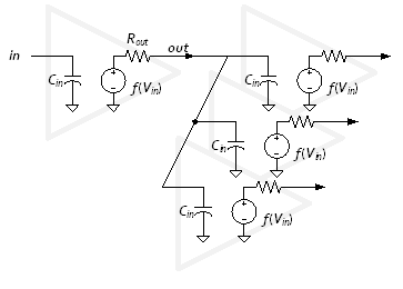
Figure 4. An example of modeling the buffer delay that varies with the external load capacitance. The CLM feature is capable of identifying the circuit group spanning multiple modules.
The CLM of XMODEL is a powerful feature that enables conservative system modeling in an event-driven logic simulator like SystemVerilog. While this may make XMODEL look almost like SPICE, using XMODEL essentially as a fast SPICE simulator is not strongly recommended especially when the highest simulation performance is desired. XMODEL is fundamentally a behavioral simulator and CLM is offered as a convenient way to describe the circuit’s behavior using conservative system description. For transistor-level circuit simulation, it is more appropriate to use SPICE.
CLM Primitives
The conservative circuit models can be described as a structural netlist, listing the circuit elements as the instances of CLM primitives with their terminal connections. For instance, the model of a linear amplifier with finite input and output resistance is listed in Figure 5.
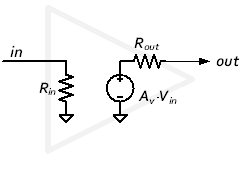
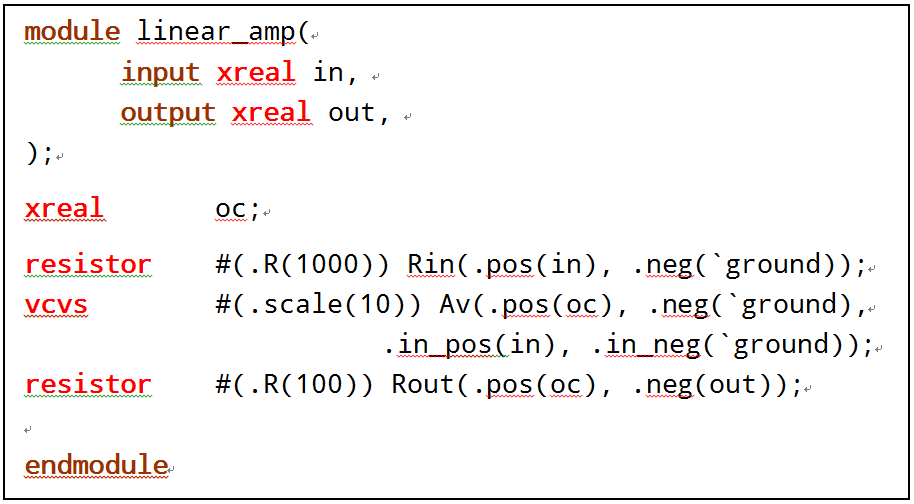
Figure 5. The conservative circuit model of a linear amplifier with finite input and output resistances using the CLM feature in XMODEL.
First, the signal nodes in the circuit are defined as xreal types. Second, the circuit is described as a structural netlist consisting of its elements, using the CLM primitives such as resistor and vcvs.
Some of the currently available CLM primitives are listed in Table 1. The supported primitives include linear elements such as resistor, inductor, and capacitor, nonlinear elements such as switch, diode, and transistors, and distributed elements such as single-conductor and multi-conductor transmission lines. The detailed description regarding the usage of these primitives can be found in the XMODEL Reference Manual.
Table 1. Available circuit-level modeling primitives.
| Circuit Elements | Description |
| resistor | Linear resistor element |
| inductor | Linear inductor element |
| capacitor | Linear capacitor element |
| res_var | Nonlinear resistor element |
| ind_var | Nonlinear inductor element |
| cap_var | Nonlinear capacitor element |
| impedance | Impedance circuit element |
| transformer | Ideal transformer circuit element |
| minductor | Mutual inductor element |
| vsource | Independent voltage source |
| isource | Independent current source |
| vcvs | Voltage-controlled voltage source |
| vccs | Voltage-controlled current source |
| ccvs | Current-controlled voltage source |
| cccs | Current-controlled current source |
| switch | Ideal switch |
| diode | Diode |
| vlimit | Voltage limiting element |
| ilimit | Current limiting element |
| nmosfet | n-type MOS transistor |
| pmosfet | p-type MOS transistor |
| npn | NPN bipolar transistor |
| pnp | PNP bipolar transistor |
| tline | Single-conductor, two-port transmission line element |
| mtline | Multi-conductor, multi-port transmission line element |
| stline | Generalized multi-conductor, multi-port transmission line element with per-port characteristic impedance and split-delay transfer functions |
As explained in Section 2, the CLM primitives are pseudo modules, which are used only to identify the isolated conservative circuit groups included in the overall system model and extract their corresponding signal-flow models. They do not implement the behaviors of the corresponding circuit elements by themselves.
CLM Interfacing with Signal-Flow Models
The signals in the signal-flow models may be connected to the conservative circuit models either as inputs or outputs. This section describes how to make connections between the conservative circuit models described with CLM primitives with the rest of the signal-flow models.
Explicit Connection Method
The most basic yet versatile way of making signal connections into and out of the conservative circuit groups is to use vsource/isource primitives and vprobe/iprobe primitives.
The vsource or isource primitive, when used with the mode “in”, drives an external xreal-typed signal into a circuit group as a voltage between its two terminals or current through them, respectively. Likewise, the vprobe or iprobe primitive measures a voltage between two terminals or current through them and drives its output with the corresponding signal, respectively. An example of using the source and probe primitives is illustrated in Figure 6.
This explicit connection method is the most versatile method as it can drive and measure voltages or currents across any two nodes or branches in the circuit.
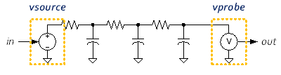
Figure 6. An example using source and probe primitives to drive and read voltages in the circuit model.
Implicit Connection Method
If the signal being driven into or measured from the circuit model is a voltage referenced to the global ground (defined as `ground), then one can make a connection without an explicit vsource or vprobe primitive. Figure 7 illustrates the case of using this implicit connection method. It has the same effect as the example in Figure 6.
Note that if the signal being driven into or measured from the circuit is not a voltage or not referenced to the global ground, one must use the explicit connection method with source and probe primitives.
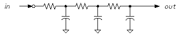
Figure 7. An example of using the implicit connection method to drive and measure voltages in the circuit model.